Overview and Tutorial

Introduction

This module provides tools for representing, manipulating, and simulating Gaussian random variables numerically. It can deal with individual variables or arbitrarily large sets of variables, correlated or uncorrelated. It also supports complicated (Python) functions of Gaussian variables, automatically propagating uncertainties and correlations through the functions.

A Gaussian variable x represents a Gaussian probability distribution, and is therefore completely characterized by its mean x.mean and standard deviation x.sdev. They are used to represent quantities whose values are uncertain: for example, the mass, 125.7±0.4 GeV, of the recently discovered Higgs boson from particle physics. The following code illustrates a (very) simple application of gvar; it calculates the Higgs boson’s energy when it carries momentum 50±0.15 GeV.

>>> import gvar as gv
>>> m = gv.gvar(125.7, 0.4)             # Higgs boson mass
>>> p = gv.gvar(50, 0.15)               # Higgs boson momentum
>>> E = (p ** 2 +  m ** 2) ** 0.5       # Higgs boson energy
>>> print(m, E)
125.70(40) 135.28(38)
>>> print(E.mean, '±', E.sdev)
135.279303665 ± 0.375787639425

Here method gvar.gvar() creates objects m and p of type gvar.GVar that represent Gaussian random variables for the Higgs mass and momentum, respectively. The energy E computed from the mass and momentum must, like them, be uncertain and so is also an object of type gvar.GVar — with mean E.mean=135.28 and standard deviation E.sdev=0.38. (Note that gvar uses the compact notation 135.28(38) to represent a Gaussian variable, where the number in parentheses is the uncertainty in the corresponding rightmost digits of the quoted mean value.)

A highly nontrivial feature of gvar.GVars is that they automatically track statistical correlations between different Gaussian variables. In the Higgs boson code above, for example, the uncertainty in the energy is due mostly to the initial uncertainty in the boson’s mass. Consequently statistical fluctuations in the energy are strongly correlated with those in the mass, and largely cancel, for example, in the ratio:

>>> print(E / m)
1.07621(64)

The ratio is 4–5 times more accurate than the either the mass or energy separately.

The correlation between m and E is obvious from their covariance and correlation matrices, both of which have large off-diagonal elements:

>>> print(gv.evalcov([m, E]))           # covariance matrix
[[ 0.16        0.14867019]
[ 0.14867019  0.14121635]]
>>> print(gv.evalcorr([m, E]))          # correlation matrix
[[ 1.          0.98905722]
 [ 0.98905722  1.        ]]

The correlation matrix shows that there is a 98.9% statistical correlation between the mass and energy.

A extreme example of correlation arises if we reconstruct the Higgs boson’s mass from its energy and momentum:

>>> print((E ** 2 - p ** 2) / m ** 2)
1 ± 1.4e-18

The numerator and denominator are completely correlated, indeed identical to machine precision, as they should be. This works only because gvar.GVar object E knows that its uncertainty comes from the uncertainties associated with variables m and p.

We can verify that the uncertainty in the Higgs boson’s energy comes mostly from its mass by creating an error budget for the Higgs energy (and for its energy to mass ratio):

>>> inputs = {'m':m, 'p':p}             # sources of uncertainty
>>> outputs = {'E':E, 'E/m':E/m}        # derived quantities
>>> print(gv.fmt_errorbudget(outputs=outputs, inputs=inputs))
Partial % Errors:
                   E       E/m
------------------------------
        p:      0.04      0.04
        m:      0.27      0.04
------------------------------
    total:      0.28      0.06

For each output (E and E/m), the error budget lists the contribution to the total uncertainty coming from each of the inputs (m and p). The total uncertainty in the energy is ±0.28%, and almost all of that comes from the mass — only ±0.04% comes from the uncertainty in the momentum. The two sources of uncertainty contribute equally, however, to the ratio E/m, which has a total uncertainty of only 0.06%.

This example is relatively simple. Module gvar, however, can easily handle thousands of Gaussian random variables and all of their correlations. These can be combined in arbitrary arithmetic expressions and/or fed through complicated (pure) Python functions, while the gvar.GVars automatically track uncertainties and correlations for and between all of these variables. The code for tracking correlations is the most complex part of the module’s design, particularly since this is done automatically, behind the scenes.

What follows is a tutorial showing how to create gvar.GVars and manipulate them to solve common problems in error propagation. Another way to learn about gvar is to look at the case studies later in the documentation. Each focuses on a single problem, and includes the full code and data, to allow for further experimentation.

gvar was originally written for use by the lsqfit module, which does multidimensional (Bayesian) least-squares fitting. It used to be distributed as part of lsqfit, but is now distributed separately because it is used by other modules (e.g., vegas for multidimensional Monte Carlo integration).

About Printing: The examples in this tutorial use the print function as it is used in Python 3. Drop the outermost parenthesis in each print statement if using Python 2; or add

from __future__ import print_function

at the start of your file.

Gaussian Random Variables

The Higgs boson mass (125.7±0.4 GeV) from the previous section is an example of a Gaussian random variable. As discussed above, such variables x represent Gaussian probability distributions, and therefore are completely characterized by their mean x.mean and standard deviation x.sdev. A mathematical function f(x) of a Gaussian variable is defined as the probability distribution of function values obtained by evaluating the function for random numbers drawn from the original distribution. The distribution of function values is itself approximately Gaussian provided the standard deviation x.sdev of the Gaussian variable is sufficiently small (and the function is sufficiently smooth). Thus we can define a function f of a Gaussian variable x to be a Gaussian variable itself, with

f(x).mean = f(x.mean)
f(x).sdev = x.sdev |f'(x.mean)|,

which follows from linearizing the x dependence of f(x) about point x.mean. This formula, together with its multidimensional generalization, lead to a full calculus for Gaussian random variables that assigns Gaussian- variable values to arbitrary arithmetic expressions and functions involving Gaussian variables. This calculus, which is built into gvar, provides the rules for standard error propagation — an important application of Gaussian random variables and of the gvar module.

A multidimensional collection x[i] of Gaussian variables is characterized by the means x[i].mean for each variable, together with a covariance matrix cov[i, j]. Diagonal elements of cov specify the standard deviations of different variables: x[i].sdev = cov[i, i]**0.5. Nonzero off-diagonal elements imply correlations (or anti-correlations) between different variables:

cov[i, j] = <x[i]*x[j]>  -  <x[i]> * <x[j]>

where <y> denotes the expectation value or mean for a random variable y.

Creating Gaussian Variables

Objects of type gvar.GVar are of two types: 1) primary gvar.GVars that are created from means and covariances using gvar.gvar(); and 2) derived gvar.GVars that result from arithmetic expressions or functions involving gvar.GVars. The primary gvar.GVars are the primordial sources of all uncertainties in a gvar code. A single (primary) gvar.GVar is created from its mean xmean and standard deviation xsdev using:

x = gvar.gvar(xmean, xsdev).

This function can also be used to convert strings like "-72.374(22)" or "511.2 ± 0.3" into gvar.GVars: for example,

>>> import gvar
>>> x = gvar.gvar(3.1415, 0.0002)
>>> print(x)
3.14150(20)
>>> x = gvar.gvar("3.1415(2)")
>>> print(x)
3.14150(20)
>>> x = gvar.gvar("3.1415 ± 0.0002")
>>> print(x)
3.14150(20)

Note that x = gvar.gvar(x) is useful when you are unsure whether x is initially a gvar.GVar or a string representing a gvar.GVar. Note also that '±' in the above example could be replaced by '+/-' or '+-'.

gvar.GVars are usually more interesting when used to describe multidimensional distributions, especially if there are correlations between different variables. Such distributions are represented by collections of gvar.GVars in one of two standard formats: 1) numpy arrays of gvar.GVars (any shape); or, more flexibly, 2) Python dictionaries whose values are gvar.GVars or arrays of gvar.GVars. Most functions in gvar that handle multiple gvar.GVars work with either format, and if they return multidimensional results do so in the same format as the inputs (that is, arrays or dictionaries). Any dictionary is converted internally into a specialized (ordered) dictionary of type gvar.BufferDict, and dictionary-valued results are also gvar.BufferDicts.

To create an array of gvar.GVars with mean values specified by array xmean and covariance matrix xcov, use

x = gvar.gvar(xmean, xcov)

where array x has the same shape as xmean (and xcov.shape = xmean.shape+xmean.shape). Then each element x[i] of a one-dimensional array, for example, is a gvar.GVar where:

x[i].mean = xmean[i]         # mean of x[i]
x[i].val  = xmean[i]         # same as x[i].mean
x[i].sdev = xcov[i, i]**0.5  # std deviation of x[i]
x[i].var  = xcov[i, i]       # variance of x[i]

As an example,

>>> x, y = gvar.gvar([0.1, 10.], [[0.015625, 0.24], [0.24, 4.]])
>>> print('x =', x, '   y =', y)
x = 0.10(13)    y = 10.0(2.0)

makes x and y gvar.GVars with standard deviations sigma_x=0.125 and sigma_y=2, and a fairly strong statistical correlation:

>>> print(gvar.evalcov([x, y]))     # covariance matrix
[[ 0.015625  0.24    ]
 [ 0.24      4.      ]]
>>> print(gvar.evalcorr([x, y]))    # correlation matrix
[[ 1.    0.96]
 [ 0.96  1.  ]]

Here functions gvar.evalcov() and gvar.evalcorr() compute the covariance and correlation matrices, respectively, of the list of gvar.GVars in their arguments.

gvar.gvar() can also be used to convert strings or tuples stored in arrays or dictionaries into gvar.GVars: for example,

>>> garray = gvar.gvar(['2(1)', '10±5', (99, 3), gvar.gvar(0, 2)])
>>> print(garray)
[2.0(1.0) 10.0(5.0) 99.0(3.0) 0 ± 2.0]
>>> gdict = gvar.gvar(dict(a='2(1)', b=['10±5', (99, 3), gvar.gvar(0, 2)]))
>>> print(gdict)
{'a': 2.0(1.0),'b': array([10.0(5.0), 99.0(3.0), 0 ± 2.0], dtype=object)}

If the covariance matrix in gvar.gvar is diagonal, it can be replaced by an array of standard deviations (square roots of diagonal entries in cov). The example above without correlations, therefore, would be:

>>> x, y = gvar.gvar([0.1, 10.], [0.125, 2.])
>>> print('x =', x, '   y =', y)
x = 0.10(12)    y = 10.0(2.0)
>>> print(gvar.evalcov([x, y]))     # covariance matrix
[[ 0.015625  0.      ]
 [ 0.        4.      ]]
>>> print(gvar.evalcorr([x, y]))    # correlation matrix
[[ 1.  0.]
 [ 0.  1.]]

gvar.GVar Arithmetic and Functions

The gvar.GVars discussed in the previous section are all primary gvar.GVars since they were created by specifying their means and covariances explicitly, using gvar.gvar(). What makes gvar.GVars particularly useful is that they can be used in arithmetic expressions (and numeric pure-Python functions), just like Python floats. Such expressions result in new, derived gvar.GVars whose means, standard deviations, and correlations are determined from the covariance matrix of the primary gvar.GVars. The automatic propagation of correlations through arbitrarily complicated arithmetic is an especially useful feature of gvar.GVars.

As an example, again define

>>> x, y = gvar.gvar([0.1, 10.], [0.125, 2.])

and set

>>> f = x + y
>>> print('f =', f)
f = 10.1(2.0)

Then f is a (derived) gvar.GVar whose variance f.var equals

df/dx cov[0, 0] df/dx + 2 df/dx cov[0, 1] df/dy + ... = 2.0039**2

where cov is the original covariance matrix used to define x and y (in gvar.gvar). Note that while f and y separately have 20% uncertainties in this example, the ratio f/y has much smaller errors:

>>> print(f / y)
1.010(13)

This happens, of course, because the errors in f and y are highly correlated — the error in f comes mostly from y. gvar.GVars automatically track correlations even through complicated arithmetic expressions and functions: for example, the following more complicated ratio has a still smaller error, because of stronger correlations between numerator and denominator:

>>> print(gvar.sqrt(f**2 + y**2) / f)
1.4072(87)
>>> print(gvar.evalcorr([f, y]))
[[ 1.          0.99805258]
 [ 0.99805258  1.        ]]
>>> print(gvar.evalcorr([gvar.sqrt(f**2 + y**2), f]))
[[ 1.         0.9995188]
 [ 0.9995188  1.       ]]

The gvar module defines versions of the standard Python mathematical functions that work with gvar.GVar arguments. These include: exp, log, sqrt, sin, cos, tan, arcsin, arccos, arctan, arctan2, sinh, cosh, tanh, arcsinh, arccosh, arctanh, erf, fabs, abs. Numeric functions defined entirely in Python (i.e., pure-Python functions) will likely also work with gvar.GVars.

Numeric functions implemented by modules using low-level languages like C will not work with gvar.GVars. Such functions must be replaced by equivalent code written directly in Python. In some cases it is possible to construct a gvar.GVar-capable function from low-level code for the function and its derivative. For example, the following code defines a new version of the standard Python error function that accepts either floats or gvar.GVars as its argument:

import math
import gvar

def erf(x):
    if isinstance(x, gvar.GVar):
        f = math.erf(x.mean)
        dfdx = 2. * math.exp(- x.mean ** 2) / math.sqrt(math.pi)
        return gvar.gvar_function(x, f, dfdx)
    else:
        return math.erf(x)

Here function gvar.gvar_function() creates the gvar.GVar for a function with mean value f and derivative dfdx at point x. A more complete version of erf is included in gvar. Note that gvar.gvar_function() also works for functions of multiple variables. See Case Study: Creating an Integrator for a less trivial application.

Some sample numerical analysis codes, adapted for use with gvar.GVars, are described in Numerical Analysis Modules in gvar.

Arithmetic operators + - * / ** == != <> += -= *= /= are all defined for gvar.GVars. Comparison operators are also supported: == != > >= < <=. They are applied to the mean values of gvar.GVars: for example, gvar.gvar(1,1) == gvar.var(1,2) is true, as is gvar.gvar(1,1) > 0. Logically x>y for gvar.GVars should evaluate to a boolean-valued random variable, but such variables are beyond the scope of this module. Comparison operators that act only on the mean values make it easier to implement pure-Python functions that work with either gvar.GVars or floats as arguments.

Implementation Notes: Each gvar.GVar keeps track of three pieces of information: 1) its mean value; 2) its derivatives with respect to the primary gvar.GVars (created by gvar.gvar()); and 3) the location of the covariance matrix for the primary gvar.GVars. The standard deviations and covariances for all gvar.GVars originate with the primary gvar.GVars: any gvar.GVar z satisfies

z = z.mean + sum_p (p - p.mean) * dz/dp

where the sum is over all primary gvar.GVars p. gvar uses this expression to calculate covariances from the derivatives, and the covariance matrix of the primary gvar.GVars. The derivatives for derived gvar.GVars are computed automatically, using automatic differentiation.

The derivative of a gvar.GVar f with respect to a primary gvar.GVar x is obtained from f.deriv(x). A list of derivatives with respect to all primary gvar.GVars is given by f.der, where the order of derivatives is the same as the order in which the primary gvar.GVars were created.

A gvar.GVar can be constructed at a very low level by supplying all the three essential pieces of information — for example,

f = gvar.gvar(fmean, fder, cov)

where fmean is the mean, fder is an array where fder[i] is the derivative of f with respect to the i-th primary gvar.GVar (numbered in the order in which they were created using gvar.gvar()), and cov is the covariance matrix for the primary gvar.GVars (easily obtained from gvar.gvar.cov).

Error Budgets from gvar.GVars

It is sometimes useful to know how much of the uncertainty in a derived quantity is due to a particular input uncertainty. Continuing the example above, for example, we might want to know how much of fs standard deviation is due to the standard deviation of x and how much comes from y. This is easily computed:

>>> x, y = gvar.gvar([0.1, 10.], [0.125, 2.])
>>> f = x + y
>>> print(f.partialsdev(x))        # uncertainty in f due to x
0.125
>>> print(f.partialsdev(y))        # uncertainty in f due to y
2.0
>>> print(f.partialsdev(x, y))     # uncertainty in f due to x and y
2.00390244274
>>> print(f.sdev)                  # should be the same
2.00390244274

This shows, for example, that most (2.0) of the uncertainty in f (2.0039) is from y.

gvar provides a useful tool for compiling an “error budget” for derived gvar.GVars relative to the primary gvar.GVars from which they were constructed: continuing the example above,

>>> outputs = {'f':f, 'f/y':f/y}
>>> inputs = {'x':x, 'y':y}
>>> print(gvar.fmt_values(outputs))
Values:
                f/y: 1.010(13)
                  f: 10.1(2.0)

>>> print(gvar.fmt_errorbudget(outputs=outputs, inputs=inputs))
Partial % Errors:
                 f/y         f
------------------------------
        y:      0.20     19.80
        x:      1.24      1.24
------------------------------
    total:      1.25     19.84

This shows y is responsible for 19.80% of the 19.84% uncertainty in f, but only 0.2% of the 1.25% uncertainty in f/y. The total uncertainty in each case is obtained by adding the x and y contributions in quadrature.

Formatting gvar.GVars for Printing/Display

gvar.GVars can be formatted analogously to floats:

>>> x =  gvar.gvar(3.14159, 0.0236)
>>> print(f'{x:.2g}', f'{x:.3f}', f'{x:.4e}', f'{x:.^20.2g}')
3.1(0) 3.142(24) 3.1416(236)e+00 .......3.1(0).......

There are also two formats, 'p' and 'P', that are specific to gvar.GVars. For these the precision field in the format specifies the number of digits displayed in the standard deviation:

>>> print(f'{x:.2p}', f'{x:.3P}')
3.142(24) 3.1416 ± 0.0236

The 'P' format always uses the ± representation of a gvar.GVar.

The '#p' format is a variation on the 'p' format. When the standard deviation is larger in magnitude than the mean, the '#p' format adjusts the precision so that at least one non-zero digit of the mean is included in the formatted string:

>>> y = gvar.gvar(0.023, 10.2)
>>> print(f'{y:.2p}', f'{y:#.2p}')
0(10) 0.02(10.20)

The default format specification is #.2p:

>>> print(f'{y}', str(y))
0.02(10.20) 0.02(10.20)

Multiple gvar.GVars in an array, or in a dictionary whose values are gvar.GVars or arrays of gvar.GVars can be formatted using gvar.fmt():

>>> print(gvar.fmt(dict(a=x, b=y), format='{:.3P}'))
{'a': '3.1416 ± 0.0236', 'b': '0.023 ± 10.2'}

Each gvar.GVar is replaced by its formatted string.

The default format can be changed using the gvar.GVar.set() method:

>>> old_settings = gvar.GVar.set(default_format='{:.2P}')
>>> print(f'{y}', str(y))
0.023 ± 10 0.023 ± 10

The original default is restored here by gvar.GVar.set(**old_settings).

gvar.GVar.set() can also be used to replace the formatter with a different function. The following example switches to a format that would work in a LaTeX document:

>>> def new_formatter(g, spec=''):
...     return r'${g.mean:{spec}}\,\pm\,{g.sdev:{spec}}$'.format(g=g, spec=spec)
...
>>> old_settings = gvar.GVar.set(formatter=new_formatter)
>>> print(y)
$0.023\,\pm\,10.2$
>>> print(f'{y:.0f}')
$0\,\pm\,10$

Again gvar.GVar.set(**old_settings) restores the original formatter.

Storing gvar.GVars for Later Use

Storing gvar.GVars in a file for later use is complicated by the need to capture the covariances between different gvar.GVars as well as their means. The easiest way to save an array or dictionary or other object g that contains gvar.GVars is to use gvar.dump(): for example,

>>> gvar.dump(g, 'gfile.pkl')

saves the data from g in a Python pickle file named 'gfile.pkl'. To reassemble the the data from g we use:

>>> g = gvar.load('gfile.pkl')

Functions gvar.dump() and gvar.load() are similar to the corresponding functions in Python’s pickle module but they preserve information about the correlations between different gvar.GVars in g. Correlations with gvar.GVars that are not in g are lost, so it is important to include all gvar.GVars of interest in g before saving them.

gvar.GVars can also be pickled easily if they are stored in a gvar.BufferDict since this data type has explicit support for pickling that preserves correlations. So if g is a gvar.BufferDict containing gvar.GVars (and/or arrays of gvar.GVars),

>>> import pickle
>>> pickle.dump(g, open('gfile.pkl', 'wb'))

saves the contents of g to a file named gfile.pkl, and the gvar.GVars are retrieved using

>>> g = pickle.load(open('gfile.pkl', 'rb'))

Of course, gvar.dump(g, 'gfile.pkl') and g = gvar.load('gfile.pkl') are simpler and achieve the same goal.

Using pickle to pickle an object containing gvar.GVars usually generates a warning about lost correlations. This can be ignored if correlations are unimportant. If pickle must be used and correlations matter, gvar.dumps/loads can sometimes be used to make this possible. Consider, for example, a class A that stores gvar.GVars a and b. We might be able to modify it so that pickle uses the gvar routines: for example, the code

class A:
    def __init__(self, a, b):
        if isinstance(a, bytes):
            self.__dict__ = gv.loads(a)
        else:
            self.a = a
            self.b = b
            ...

    def __reduce__(self):
        return A, (gv.dumps(self.__dict__), None)

    ...

has pickle convert the class’s dictionary into a byte stream using gv.dumps(self.__dict__) when pickling. This is reconstituted into a dictionary in A.__init__, using gv.loads(a), upon un-pickling.

Sampling Distributions; Non-Gaussian Expectation Values

By default functions of gvar.GVars are also gvar.GVars, but there are cases where such functions cannot be represented accurately by Gaussian distributions. The product of 0.1(4) and 0.2(5), for example, is not very Gaussian because the standard deviations are large compared to the scale over which the product changes appreciably. In such cases one may want to use the true distribution of the function, instead of its Gaussian approximation, in an analysis.

One approach to this problem is to use simulation. The following code analyzes the distribution of f(p) = sin(p[0] * p[1]) where p = [0.1(4), 0.2(5)]. To do this:

1. it generates 100,000 samples [ps[0,i], ps[1,i]], with i=0...99,999, drawn from the Gaussian distribution specified by p;

2. it calculates f(ps[:,i]) = sin(ps[0,i] * ps[1,i]) for each sample i, thereby obtaining 100,000 samples drawn from the real distribution for f(p);

3. it estimates the mean and standard deviation of this distribution from the samples.

The sampling in step #1 is done using gvar.sample():

import gvar as gv
import numpy as np

p = gv.gvar(['0.1(4)', '0.2(5)'])
def f(p):
    return np.sin(p[0] * p[1])
print(f'Gaussian approx.: {f(p)}')

# sample p, f(p) distributions
n = 100_000
ps = gv.sample(p, nbatch=n)                             # step #1
f_ps = f(ps)                                            # step #2

# Gaussian approximation from simulation samples
f_p_sim = gv.gvar(np.mean(f_ps), np.std(f_ps))          # step #3
print(f'Gaussian approx. to simulation: {f_p_sim}')

Running this code generates the following output:

Gaussian approx.: 0.020(94)
Gaussian approx. to simulation: 0.02(21)

Evaluating f(p) directly gives 0.020(94); estimating the mean and standard deviation from the samples gives 0.02(21). The means agree but the simulation gives a standard deviation that is more than twice as large, suggesting fat tails on the distribution.

Note that the line calculating f_p_sim can be simplified using gvar.gvar_from_sample():

f_p_sim = gv.gvar_from_sample(f_ps)

We can look more closely at the f(ps) distribution by examining moments and a histogram of the distribution, adding the following to the code above:

moments = np.mean([f_ps, f_ps**2, f_ps**3, f_ps**4], axis=-1)
print(f'\nMoments: {moments}')
counts, bins = np.histogram(f_ps, bins=50)
stats = gv.PDFStatistics(
    moments=moments,
    histogram=(bins, counts),
    )
print('\nSimulation statistics:')
print(stats)

This produces the following output:

Moments: [0.01876974 0.04336239 0.00491038 0.01153368]

Simulation statistics:
  mean = 0.018769738628101846   sdev = 0.20739   skew = 0.27825   ex_kurt = 3.0849
  median = -0.03372571848916756   plus = 0.16875932667218416   minus = 0.13574922445045393

The moments indicate that the distribution is slightly skewed, but has a large excess kurtosis of 3.1, which is indicative of fat tails. The histogram gives an estimate of the median, which is slightly offset from the mean, as well as estimates for the interval on either side of the median ((median-minus,median) or (median,median+plus)) that contains 34% of the probability. These intervals are again broader than what is suggested by simply evaluating f(p).

Finally we can look at the histogram for the distribution of f(p) inferred from the samples, again adding to the code above:

import matplotlib.pyplot as plt

# plot histogram of f(p) distribution
plt.stairs(counts / n, bins, fill=True, color='k', ec='k', alpha=0.25, lw=1., label='Sim.')

# compare with 2 Gaussian distributions
x = np.linspace(-1,1,500)
binsize = bins[1] - bins[0]
fmt = iter(['r--', 'b:'])
label = iter(['Gauss.', 'Gauss. Sim.'])
for f in [f(p), f_p_sim]:
    y = np.exp(-(x - f.mean)**2 / 2 / f.var) / f.sdev / (2 * np.pi) ** 0.5
    plt.plot(x, y * binsize, next(fmt), label=next(label))
plt.legend()
plt.xlabel('sin(p[0]*p[1])')
plt.ylabel('probability')
plt.show()

This generates the following figure:

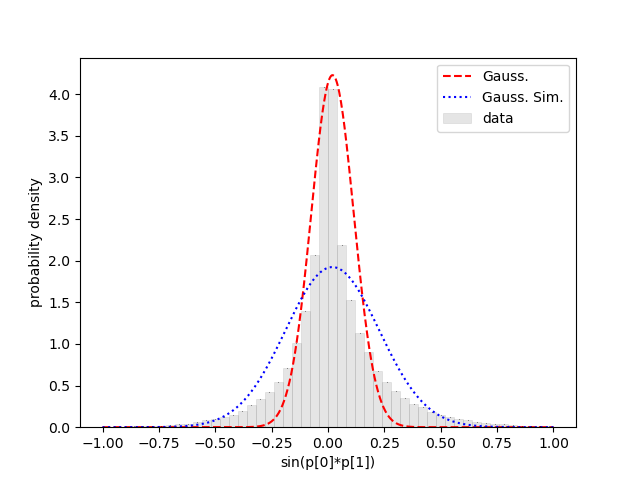
It shows the actual probability associated with each f(p) bin (gray bins), together with the shape (red dashed line) expected from the Gaussian approximation (0.020(94)). It also shows the Gaussian distribution corresponding to the correct mean and standard deviation (0.02(21)) of the distribution (blue dotted line). Neither Gaussian in this plot is quite right: the first is more accurate close to the maximum, while the second does better further out.

This example is relatively simple since the underlying Gaussian distribution is only two dimensional and uncorrelated. gvar.sample() works well in higher dimensions and with correlated gvar.GVars. gvar.sample() is implemented using gvar.raniter(), which can be used to generate a series of sample batches. Both of these functions work for distributions defined by dictionaries, as well as arrays (or individual gvar.GVars).

Note that gvar provides limited support for non-Gaussian probability distributions through the gvar.BufferDict dictionary. This is illustrated by the following code fragment:

>>> b = gv.BufferDict()
>>> b['log(x)'] = gv.gvar('1(1)')
>>> b['f(y)'] = gv.BufferDict.uniform('f', 2., 3.)
>>> print(b)
{'log(x)': 1.0(1.0), 'f(y)': 0 ± 1.0}
>>> print(b['x'], b['y'])
2.7(2.7) 2.50(40)

Even though 'x' and 'y' are not keys, b['x'] and b['y'] are defined. b['x'] is set equal to exp(b['log(x)']). In a simulation this means that values for b['log(x)'] will be drawn from a Gaussian distribution 1±1, while the values b['x'] will be drawn from the corresponding log-normal distribution. Similarly the values for b['f(y)'] are drawn from the Gaussian 0±1, while the values of b['y'] are distributed uniformly on the interval between 2 and 3. 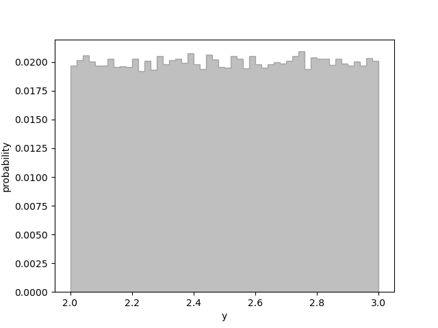Method gvar.BufferDict.uniform() defines the function f(y) that connects the Gaussian and uniform distributions. The plot produced by the code

>>> bs = gv.sample(b, nbatch=100_000)
>>> counts, bins = np.histogram(bs['y'], bins=50)
>>> plt.stairs(counts / 100_000, bins, fill=True, color='k', ec='k', alpha=0.25, lw=1.)
>>> plt.show()

shows small statistical fluctuations around a uniform probability distribution distribution:

Note finally that bootstrap copies of gvar.GVars are easily created. A bootstrap copy of gvar.GVar x ± dx is another gvar.GVar with the same width but where the mean value is replaced by a random number drawn from the original distribution. Bootstrap copies of a data set, described by a collection of gvar.GVars, can be used as new (fake) data sets having the same statistical errors and correlations:

>>> g = gvar.gvar([1.1, 0.8], [[0.01, 0.005], [0.005, 0.01]])
>>> print(g)
[1.10(10) 0.80(10)]
>>> print(gvar.evalcov(g))                  # print covariance matrix
[[ 0.01   0.005]
 [ 0.005  0.01 ]]
>>> gbs_iter = gvar.bootstrap_iter(g)
>>> gbs = next(gbs_iter)                    # bootstrap copy of f
>>> print(gbs)
[1.14(10) 0.90(10)]                         # different means
>>> print(gvar.evalcov(gbs))
[[ 0.01   0.005]                            # same covariance matrix
 [ 0.005  0.01 ]]

Such fake data sets are useful for analyzing non-Gaussian behavior, for example, in nonlinear fits.

Limitations

The most fundamental limitation of this module is that the calculus of Gaussian variables that it assumes is only valid when standard deviations are small (compared to the distances over which the functions of interest change appreciably). One way of dealing with this limitation is to use simulations, as discussed in Sampling Distributions; Non-Gaussian Expectation Values.

Another potential issue is roundoff error, which can become problematic if there is a wide range of standard deviations among correlated modes. For example, the following code works as expected:

>>> from gvar import gvar, evalcov
>>> tiny = 1e-4
>>> a = gvar(0., 1.)
>>> da = gvar(tiny, tiny)
>>> a, ada = gvar([a.mean, (a+da).mean], evalcov([a, a+da])) # = a,a+da
>>> print(ada-a)   # should be da again
0.00010(10)

Reducing tiny, however, leads to problems:

>>> from gvar import gvar, evalcov
>>> tiny = 1e-8
>>> a = gvar(0., 1.)
>>> da = gvar(tiny, tiny)
>>> a, ada = gvar([a.mean, (a+da).mean], evalcov([a, a+da])) # = a, a+da
>>> print(ada-a)   # should be da again
1(0)e-08

Here the call to gvar.evalcov() creates a new covariance matrix for a and ada = a+da, but the matrix does not have enough numerical precision to encode the size of da’s variance, which gets set, in effect, to zero. The problem arises here for values of tiny less than about 2e-8 (with 64-bit floating point numbers; tiny**2 is what appears in the covariance matrix).

Optimizations

When there are lots of primary gvar.GVars, the number of derivatives stored for each derived gvar.GVar can become rather large, potentially (though not necessarily) leading to slower calculations. One way to alleviate this problem, should it arise, is to separate the primary variables into groups that are never mixed in calculations and to use different gvar.gvar()s when generating the variables in different groups. New versions of gvar.gvar() are obtained using gvar.switch_gvar(): for example,

import gvar
...
x = gvar.gvar(...)
y = gvar.gvar(...)
z = f(x, y)
... other manipulations involving x and y ...
gvar.switch_gvar()
a = gvar.gvar(...)
b = gvar.gvar(...)
c = g(a, b)
... other manipulations involving a and b (but not x and y) ...

Here the gvar.gvar() used to create a and b is a different function than the one used to create x and y. A derived quantity, like c, knows about its derivatives with respect to a and b, and about their covariance matrix; but it carries no derivative information about x and y. Absent the switch_gvar line, c would have information about its derivatives with respect to x and y (zero derivative in both cases) and this would make calculations involving c slightly slower than with the switch_gvar line. Usually the difference is negligible — it used to be more important, in earlier implementations of gvar.GVar before sparse matrices were introduced to keep track of covariances. Note that the previous gvar.gvar() can be restored using gvar.restore_gvar(). Function gvar.gvar_factory() can also be used to create new versions of gvar.gvar().